Table Of Contents

PostGIS, SQL Server 2008 R2, Oracle 11G R2

We just completed our compare of the spatial functionality of PostgreSQL 8.4/PostGIS 1.5, SQL Server 2008 R2, Oracle 11G R2 (both its built-in Locator and Spatial add-on). Most of the compare is focused on what can be gleaned from the manual of each product.

In summary, all products have changed a bit since their prior versions. The core changes:

• PostGIS 1.5 has geodetic support now in the form of geography as well as some beefed up functions and additional distance functions like ST_ClosestPoint, ST_MaxDistance, ST_ShortestLine/LongestLine
• SQL Server 2008 R2 basic spatial support hasn't changed much when compared to SQL Server 2008, but there is a lot more integration going on integrating Spatial into reporting services, Share Point and just integration in general with SQL Server 2008 R2 and the Office 2010 stack.
• Oracle 11G R2 - has finally offered an uninstall script for Locator folks who do not care to break the law by accidentally using functions only licensed in Oracle spatial, but innocently exposed in Oracle Locator. If all that were not great enough, you are now allowed to legally do a centroid if you are using Oracle Locator. Doing unions, intersections, and differences is still a legal no no for Oracle Locator folks. Oracle now provides Affine transform functions, which have long been provided by PostGIS and have been available via the MPL licensed CLR Spatial package of SQL Server 2008.

I still haven't figured out where this R2 convention started. I thought it was just a Microsoft thing, but I see Oracle follows the same convention as well.

PostGIS in Action book news

We are working on polishing off some suggestions in our last round of reviews and also incorporating changes from earlier reviews. We got perfect ratings in our last round. We also got two very rave blog reviews which we were pretty excited to read. One from Bill Dollins A Look at "PostGIS in Action" and Mark Leslie PostGIS in Action. It is always nice to know people appreciate your writing or even if they find flaws in it, have interest in it enough to comment about it. It makes all the effort worth while.

PostGIS in Action is available for Pre-Order on Amazon or Direct from Manning. The benefit of ordering direct from Manning is that you get the e-Book draft copy now and updates as we revise the chapters. The benefit of ordering from Amazon is that you can lock in a lower price. The price of our book on Amazon has been slashed significantly to $33.74 USD from its original $49.99 price with a pre-order price guarantee. I get a bit of a chuckle out of the fact that PostGIS in Action is ranked number 94 (at least for the moment) on Amazone in "Books > Computers & Internet > Hardware > Handheld & Mobile Devices" along side all those iPad application and Android books. I didn't even think of that as a market that PostGIS/PostgreSQL compete heavily in.

PostgreSQL 9.0 beta 2 just got released this week. We may see another beta before 9.0 is finally released, but it looks like PostgreSQL 9.0 will be here probably sometime this month. Robert Treat has a great slide presentation showcasing all the new features. The slide share for those on Robert Treat's slide share page.

We'll list the key ones with our favorites at the top:

Our favorites

1. The window function functionality has been enhanced to support ROWS PRECEDING and FOLLOWING. Recall we discussed this in Running totals and sums using PostgreSQL 8.4 a hack for getting around the lack of ROWS x PRECEDING and FOLLOWING. No more need for that. This changes our comparison we did Window Functions Comparison Between PostgreSQL 8.4, SQL Server 2008, Oracle, IBM DB2. Now the syntax is inching even closer to Oracle's window functionality, far superior to SQL Server 2005/2008, and about on par with IBM DB2. We'll do updated compare late this month or early next month. Depesz has an example of this in Waiting for 9.0 – extended frames for window functions
2. Ordered Aggregates. This is extremely useful for spatial aggregates and ARRAY_AGG, STRING_AGG, and medians where you care about the order of the aggregation. Will have to give it a try. For example if you are building a linestring using ST_MakeLine, a hack you normally do would be to order your dataset a certain way and then run ST_MakeLine. This will allow you to do ST_MakeLine(pt_geom ORDER BY track_time) or ARRAY_AGG(student ORDER BY score) This is very very cool. Depesz has some examples of ordered aggregates.
3. Join removal -- this is a feature that will remove joins from the execution plans where they are not needed. For example where you have a left join that doesn't appear in a where or as a column in select. This is important for people like us that rely on views to allow less skilled users to be able to write meaningful queries without knowing too much about joins or creating ad-hoc query tools that allow users to pick from multiple tables. Check out Robert Haas why join removal is cool for more use cases.
4. GRANT/REVOKE ON ALL object IN SCHEMA and ALTER DEFAULT PRIVILEGES. This is just a much simpler user-friendly way of applying permissions. I can't tell you how many times we get beat up by MySQL users who find the PostgreSQL security management tricky and tedious to get right. Of course you can count on Depesz to have an example of this too Waiting for 9.0 - GRANT ALL

Runner ups

1. pg_upgrade is now included in contrib and much improved we hear. Can't wait to try this out. This will allow for in-place migration from PostgreSQL 8.3+ -> 9.0
2. Streaming replication, Hot standby more details Built-in replication in PostgreSQL 9.0
3. STRING_AGG -- this is a nice to have so you don't need to do array_to_string(ARRAY_AGG(somefield), '\') and with the ORDER BY feature its even better.
4. Conditional triggers - triggers that only run based on some boolean expression. Improves trigger speed by a bit for some kinds of triggers
5. ANSI SQL column level triggers
6. DROP IF EXISTS for columns and constraints
7. Python 3 support - now you can write database stored functions in PL/Python 3 as well as the 2.5/2.6 series.
8. Explain plan improvements -- now you can see shared buffers using EXPLAIN (ANALYZE, buffers) SELECT * FROM sometable;
9. DO it -- run anonymous PL functions subroutines. Useful for one off kind of stuff or mixing various languages in a work process.
10. Windows 64-bit support
11. exclusion constraints - this is useful for schedules and so forth to prevent overlapping periods. Jeff Davis has some slides up on how this works. Not Just Unique.
12. other stuff

Another new feature is the GUC for outputting bytea data as HEX or ESCAPED. The default is now HEX. This has broken our ability to display geometries using OpenJump ad-hoc query tool unless we do a work-around of ALTER DATABASE gisdb SET bytea_output='escape';. We are still not quite sure how much of an issue this is. PostgreSQL 9.0 ST_AsBinary rendering

One of the coolest features of PostgreSQL is the ability to write functions using plain old SQL. This feature it has had for a long time. Even before PostgreSQL 8.2. No other database to our knowledge has this feature. By SQL we mean sans procedural mumbo jumbo like loops and what not. This is cool for two reasons:

• Plain old SQL is the simplest to write and most anyone can write one and is just what the doctor ordered in many cases. PostgreSQL even allows you to write aggregate functions with plain old SQL. Try to write an aggregate function in SQL Server you've got to pull out your Visual Studio this and that and do some compiling and loading and you better know C# or VB.NET. Try in MySQL and you better learn C. Do the same in PostgreSQL (you have a large choice of languages including SQL) and the code is simple to write. Nevermind with MySQL and SQL Server, you aren't even allowed to do those type of things on a shared server or a server where the IT department is paranoid. The closest with this much ease would be Oracle, which is unnecessarily verbose.
• Most importantly -- since it is just SQL, for simple user-defined functions, a PostgreSQL sql function can often be in-lined into the overall query plan since it only uses what is legal in plain old SQL.

This inlining feature is part of the secret sauce that makes PostGIS fast and easy to use. So instead of writing geom1 && geom2 AND Intersects(geom1,geom2) -- a user can write ST_Intersects(geom1,geom2) . The short-hand is even more striking when you think of the ST_DWithin function.

With an inlined function, the planner has visibility into the function and breaks apart the spatial index short-circuit test && from the more exhaustive absolute test Intersects(geom1,geom2) and has great flexibility in reordering the clauses in the plan.

In PostGIS 1.5, we accidentally broke this secret sauce for Geography ST_Intersects and ST_Covers, ST_CoveredBy by putting in a STRICT clause in our SQL function declaration as documented in our bug ticket. So a query that would normally take 50 ms to run was taking 10 seconds.

There is nothing we could find that suggests STRICT should have this effect. Is it by design in PostgreSQL or a bug? STRICT should in theory ensure that any input going into a function that is NULL should result in a NULL output, but how does this translate to loss of transparency?

To demonstrate difference in what the plans look like, how you can tell planner is loosing visibility into the function. We will create our dummy data set.

-- create dummy PostGIS geography data --
CREATE TABLE geogtest(gid SERIAL primary key, geog geography(POLYGON,4326));
CREATE INDEX idx_geogtest_geog
  ON geogtest
  USING gist
  (geog);
  
INSERT INTO geogtest(geog)
SELECT ST_Buffer(geog,random()*10) As geog
FROM (SELECT ST_GeogFromText('POINT(' || i*0.5 || ' ' || j*0.5 || ')') As geog
    FROM generate_series(-350,350) As i 
        CROSS JOIN generate_series(-175,175) As j
        ) As foo
LIMIT 1000;

vacuum analyze geogtest;

Then we create two versions of our function, one with STRICT and one without STRICT. The functions are otherwise exactly the same.

-- create our 2 intersects functions  -- 
CREATE OR REPLACE FUNCTION ST_IntersectsBlackBox(geography, geography)
  RETURNS boolean AS
$$
SELECT $1 && $2 AND _ST_Distance($1, $2, 0.0, false) < 0.00001
$$
  LANGUAGE 'sql' IMMUTABLE STRICT;
  
CREATE OR REPLACE FUNCTION ST_IntersectsTransparent(geography, geography)
  RETURNS boolean AS
$$
SELECT $1 && $2 AND _ST_Distance($1, $2, 0.0, false) < 0.00001
$$
  LANGUAGE 'sql' IMMUTABLE;  

Then we test them out.

-- THE BIG BAD BLACK, UGLY, AND SLOW ---
SELECT f.gid as gid1, count(f2.gid) As tot
FROM geogtest As f INNER JOIN geogtest As f2
    ON ST_IntersectsBlackBox(f.geog, f2.geog)
GROUP BY f.gid;

-- takes 5775 - 6000 ms on PostgreSQL 9.0 beta 1 - similar for 8.4 and 8.3
-- Explain analyze 
QUERY PLAN
-----------------------------------------------------------------------------------------------------------------
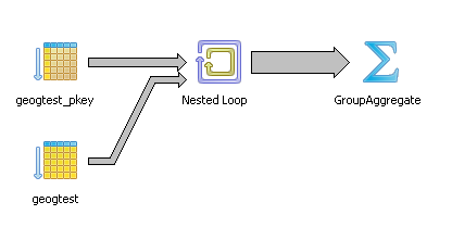
 GroupAggregate  (cost=0.00..348794.42 rows=1000 width=8) (actual time=6.850..6720.039 rows=1000 loops=1)
   ->  Nested Loop  (cost=0.00..347115.25 rows=333333 width=8) (actual time=0.102..6717.928 rows=1000 loops=1)
         Join Filter: st_intersectsblackbox(f.geog, f2.geog)
         ->  Index Scan using geogtest_pkey on geogtest f  (cost=0.00..115.25 rows=1000 width=2308) (actual time=0.014..1.039 rows=1000 loops=1)
         ->  Seq Scan on geogtest f2  (cost=0.00..87.00 rows=1000 width=2308) (actual time=0.001..0.443 rows=1000 loops=1000)
 Total runtime: 6720.376 ms

-- THE BEAUTIFUL, FAST, and NOTHING TO HIDE --
SELECT f.gid as gid1, count(f2.gid) As tot
FROM geogtest As f INNER JOIN geogtest As f2
    ON ST_IntersectsTransparent(f.geog, f2.geog)
GROUP BY f.gid;

-- Takes 48 ms on PostgreSQL 9.0 beta 1 - similar for 8.4 and 8.3
-- Explain analyze 
QUERY PLAN
--------------------------------------------------------------------------------
 HashAggregate  (cost=970.52..983.02 rows=1000 width=8) (actual time=34.100..34.491 rows=1000 loops=1)
 ->  Nested Loop  (cost=0.00..963.86 rows=1333 width=8) (actual time=0.205..33.154 rows=1000 loops=1)
       Join Filter: (_st_distance(f.geog, f2.geog, 0::double precision, false) < 1e-005::double precision)
       ->  Seq Scan on geogtest f  (cost=0.00..87.00 rows=1000 width=2308) (actual time=0.009..0.619 rows=1000 loops=1)
       ->  Index Scan using idx_geogtest_geog on geogtest f2  (cost=0.00..0.61rows=1 width=2308) (actual time=0.025..0.026 rows=1 loops=1000)
             Index Cond: (f.geog && f2.geog)
 Total runtime: 35.720 ms

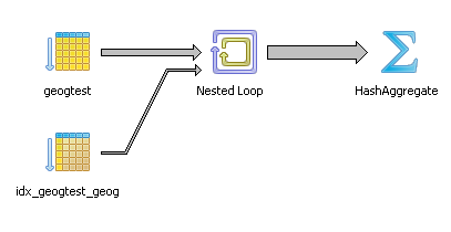
Okay there is a lot you can see yada yada yada like for those of us who lack patience and let our eyes gaze yawningly only to be mesmerized by the colors and the lines of the PgAdmin diagram - in the PgAdmin graphical picture the big fat line leading to the Group Aggregate is obviously fatter than the skinnier line leading to the Hash aggregate for the transparent one. The most important giveaway is that in the beautiful plan, we don't see the SQL function named anywhere. Its dissolved into two parts -- the spatial index condition and the more costly _ST_Distance.., but in the BIG BLACK and UGLY there it is ST_IntersectsBlackBox like a bullet-proof impenetrable vest that the planner just takes as is like a patient afraid of the surgeon's scalpel and hiding a big tumor screaming: I'm fine really, don't touch me. Nothing to see here.

Now there are certain conditions where you want your function to be a black box, like in cases when there is absolutely no way the planner can optimize it with an index scan. There is no point in wasting the planner's time allowing it to inspect it. However in these cases, we want the planner to say Ah yes I see you are using a construct that can be aided with this spatial index I have here. Let me take you apart and put you back together in a more efficient order.

I know a lot has been said about this beautiful value we affectionately call NULL, which is neither here nor there and that manages to catch many of us off guard with its casual neither here nor thereness. Database analysts who are really just back seat mathematicians in disguise like to philosophize about the unknown and pat themselves on the back when they feel they have mastered the unknown better than any one else. Of course database spatial analysts, the worst kind of back seat mathematicians, like to talk not only about NULL but about EMPTY and compare notes with their brethren and write dissertations about what to do about something that is neither here nor there but is more known than the unknown, but not quite as known as the empty string.

Okay getting to the point, one of our clients asked us about a peculiar problem they had with a query, and the strange results they were getting. We admit this still manages to catch us off guard every once in a while.

Here is a cute little example to demonstrate.

CREATE TABLE testnulls(id integer, id2 integer PRIMARY KEY);

CREATE UNIQUE INDEX uidx_testnulls_id
   ON testnulls USING btree (id);

INSERT INTO testnulls(id, id2)
SELECT 1,5 UNION ALL SELECT 2,6 UNION ALL SELECT NULL, 2;


-- wow this works
INSERT INTO testnulls(id,id2)
VALUES(null,0);



-- case 1  - returns no records
SELECT n.id2
FROM testnulls As n
WHERE n.id2 NOT IN(SELECT id FROM testnulls);

-- case 2 - returns 3 records
SELECT n.id2
FROM testnulls As n
WHERE n.id2 NOT IN(SELECT t.id FROM testnulls As t WHERE t.id IS NOT NULL);

-- case 3 -- returns 1 record
SELECT n.id2
FROM testnulls As n
WHERE n.id2 IN(SELECT t.id FROM testnulls As t );


-- case 4 -- returns 1 record
SELECT n.id2
FROM testnulls As n
WHERE n.id IN(SELECT t.id2 FROM testnulls As t );


-- case 5 -- returns 2 records
SELECT n.id, n.id2
FROM testnulls As n
WHERE n.id IN(SELECT t.id FROM testnulls As t );

Many will be surprised to find out that Case 1 yields no records and wonder how its different from case 2. Some may also wonder why case 5 does not return the records with null values. This is not a bug in PostgreSQL, but just the nature of NULL that you will see in other ANSI SQL compliant non-PostgreSQL databases as well.

The other interesting thing demonstrated by the example above, is the idea of a unique index vs. a primary key. In a primary key, you can't have nulls, but in a unique key, you can have as many nulls as you want, but other values must be unique. This is again ANSI standard compliant behavior you will see in other databases.

Why does case 1 return no records?

Since the NOT IN subquery has NULLS, which is another way of saying UNKNOWN, you can't be aboslutely sure that a value is not in the unknown set, but if asked to say true or false what do you say in such a case? The answer according to the ANSI standard is false.

Why does case 5 not return NULL records?

You can't say a missing value is equal to a set of missing or non-missing values, but should you return true or false when asked to do so? The answer according to the ANSI standard is false.

Just say NO

So in short, when in doubt about any question that requires a Yes or NO answer, just say NO.

THe STRICTNESS problem

This as odd as it may seem is also related to the STRICTNESS issue we brought up that broke the inlining logic we had in place for PostGIS functions. As Anarazel beautifully explains in our bug ticket that all boolean expressions are fundamentally considered to be not strict meaning they expect a true or false answer (not unknown). What STRICTNESS means is that when any of the inputs to your function is NULL, your answer should be NULL, but in the case of booleans, things often get messy when you ask for data and the computer answers, "I DON'T KNOW, IF I SHOULD GIVE YOU THIS DATA".

Pierre Racine has been diligently working on PostGIS WKT Raster development. He was recently creating an sql function that uses output parameters. That was all nice and well, except he couldn't figure out how to output the output parameters as columns.

The function looked something like this:

CREATE FUNCTION somefunction(rast raster, OUT field1 integer, OUT field2 sometype, etc.) AS
	$$ blah blah blah $$
LANGUAGE 'sql';

The answer I said:

Pierre said: Great that works, but how come its numoutputfields times slower than

SELECT somefunction(rast) As f 
	FROM somerastertable;

How do I get the original faster speed?

To my embarassment, I had never noticed this pattern of slowness before and I've been using this construct for years. So I suggested:

SELECT (m).* 
FROM 
 (SELECT somefunction(rast) As m 
	FROM somerastertable) As foo

That got him back to much closer speed of the original. So the morals of this story:

• It pays to be helpful
• You don't know how good it can be until someone with fresh eyes comes along and points out the flaws in your practices.

I have with this bit of information, increased our batch geocoding algorithm speed by 5-fold in some cases and of course it will help in other avenues such as the common PostGIS practice of

SELECT (ST_Dump(geom)).*
	FROM sometable

I can rewrite the above as the below and I suspect probably double my speed where I need extra speed. I still prefer the old syntax since its a bit shorter albeit slower. Where I really need to improve speed I will try this alternative syntax.

SELECT (g).geom, (g).path[1]
FROM (SELECT ST_Dump(geom) As g 
	FROM sometable) As foo

Please note that this particular issue applies to PostgreSQL 8.4 and I presume it effects below versions as well. I haven't tried this in PostgreSQL 9.0 to see if the difference in syntax would make a difference in speed. Still need to load up all the Tiger data 2009 we have in our 8.4 install into 9.0 to test our batch geocoding processing algorithm.

For those people coming from Oracle, SQL Server and MySQL or other databases that have soundex functionality, you may be puzzled, or even frustrated when you try to do something like
WHERE soundex('Wushington') = soundex('Washington')
in PostgreSQL and get a function does not exist error.

Well it does so happen that there is a soundex function in PostgreSQL, and yes it is also called soundex, but is offered as a contrib module and not installed by default. It also has other fuzzy string matching functions in addition to soundex. One of my favorites, the levenshenstein distance function is included as well. In this article we'll be covering the contrib module packaged as fuzzystrmatch.sql. Details of the module can be found in FuzzyStrMatch. The contrib module has been around for sometime, but has changed slightly from PostgreSQL version to PostgreSQL version. We are covering the 8.4 version in this article.

For those unfamiliar with soundex, its a basic approach developed by the US Census in the 1930s as a way of sorting names by pronounciation. Read Census and Soundex for more gory history details.

Given that it is an approach designed primarily for the English alphabet, it sort of makes sense why its not built-in to PostgreSQL, which has more of a diverse international concern. For example if you used it to compare two words in Japanese or Chinese, don't think it would fair too well in any of the database platforms that support this function.

The original soundex algorithm has been improved over the years. Though its still the most common used today, newer variants exist called MetaPhone developed in the 1990s and Double Metaphone (DMetaPhone) developed in 2000 that support additional consonants in other languages such as Slavic, Celtic, Italian, Spanish etc. These two variants are also included in the fuzzystrmatch contrib library. The soundex function still seems to be the most popularly used at least for U.S. This is perhaps because most of the other databases (Oracle, SQL Server, MySQL) have soundex built-in but not the metaphone variants. So in a sense soundex is a more portable function. The other reason is that metaphone and dmetaphone take up a bit more space and are also more processor intensive to compute than soundex. We'll demonstrate some differences between them in this article.

To enable soundex and the other fuzzy string matching functions included, just run the share/contrib/fuzzystrmatch.sql located in your PostgreSQL install folder. This library is an important piece of arsenal for geocoding and genealogy tracking particularly the U.S. streets and surnames data sets. I come from a long line of Minors, Miners, Burnettes and Burnets.

For the next set of exercises, we will be using the places dataset we created in Importing Fixed width data into PostgreSQL with just PSQL.

Using Soundex

One of the useful things about soundex, metaphone, and dmetaphone functions in PostgreSQL is that you can index them to get faster performance when searching. Below is a simple example of creating a functional index with soundex and using it.

CREATE INDEX idx_places_sndx_loc_name
   ON places USING btree (soundex(loc_name));

Although the index is not necessary, it improves speed fairly significantly of queries for larger datasets. Regardless of if you add an index or not, you would use the soundex function in a construct such as below.

SELECT loc_name 
FROM places 
WHERE soundex(loc_name) = soundex('Abeville') 
ORDER BY loc_name;


-- output --
    loc_name
----------------
 Abbeville city
 Abbeville city
 Abbeville city
 Abbeville city
 Abbeville town
 Abbyville city
 Abie village

The above result wasn't too bad, but what if we try

SELECT loc_name 
FROM places 
WHERE soundex(loc_name) = soundex('rising sun')
ORDER BY loc_name;


--- results not as appealing --
       loc_name
----------------------
Racine city
Racine city
Raisin City CDP
Rawson city
Regan city
Regina CDP
Riggins city
Rising City village
Rising Star town
Rising Sun-Lebanon CDP
Rising Sun city
Rising Sun town
Risingsun village
Rison city
Rockingham city
Ruskin CDP

Metaphone

As stated soundex, is not as accurate as metaphone and dmetaphone particularly when dealing with non-English languages. If we were to try the above exercises with metaphone, how would they fair?

Metaphone takes an additional argument that defines the length of the metaphone encoding. The longer you make this the more exact the match needs to be. If we repeat our above exercise:

SELECT loc_name 
FROM places 
WHERE metaphone(loc_name,5) = metaphone('rising sun',5)
ORDER BY loc_name;



-- Result is much more appealing
       loc_name
-----------------------
Rising City village
Rising Star town
Rising Sun-Lebanon CDP
Rising Sun city
Rising Sun town
Risingsun village

If we increase our sensitivity a little more, we get fewer and fewer matches till we get nothing. For example:

SELECT loc_name 
FROM places  
WHERE metaphone(loc_name,6) = metaphone('rising sun',6)
ORDER BY loc_name;


-- Yields
        loc_name
-----------------------
 Rising Sun-Lebanon CDP
 Rising Sun city
 Rising Sun town
 Risingsun village

Double MetaPhone

There are two dmetaphone functions in Postgres. There is regular dmetaphone and dmetaphone_alt. The dmetaphone you can think of as returning the primary pronounciation and is similar to what metaphone returns. The dmetaphone_alt will return an alternative pronounciation which may or may not be different from the dmetaphone. If its a non-English word, then the two results tend to be different. For this next exercise, we'll try a slightly foreign place name.

SELECT loc_name 
FROM places
WHERE dmetaphone(loc_name) = dmetaphone('Elle Cahon')
ORDER BY loc_name;


--The above returns no answers, but if instead we use the alt --
SELECT loc_name 
FROM places  
WHERE dmetaphone_alt(loc_name) = dmetaphone_alt('Elle Cahon')
ORDER BY loc_name;



-- We get
   loc_name
---------------
 El Cajon city

If you use soundex for the above matching, you get a bunch of results, none of which are El Cajon. If you use metaphone and set sensitivity to 4, you get some results, but again none are El Cajon.

What is a levenshtein distance?

A levenshtein distance is in a nutshell a measure of how many edits you need to make to a source string to convert it to the target string. So it is the spelling distance between two words.

It is another function packaged in fuzzy string match contrib and also a common favorite for geocoding. Since one of the arguments is not constant for a given column (you are comparing two strings), you can't index it like you can soundex and other soundex variants. It is as a result often used as a secondary search filter to further rank the outputs returned by the soundex family of functions.

In its simplest form, it takes two strings and returns the number of character edits needed to convert one string to another. Below is an example use:

SELECT loc_name , levenshtein(loc_name, 'rising sun')
FROM places
WHERE soundex(loc_name) = soundex('rising sun')
ORDER BY levenshtein(loc_name, 'rising sun');


---
        loc_name        | levenshtein
------------------------+-------------
 Rising Sun city        |           7
 Rising Sun town        |           7
 Regina CDP             |           7
 Ruskin CDP             |           7
 Rison city             |           7
 Racine city            |           8
 Riggins city           |           8
 Racine city            |           8
 Rawson city            |           9
 Rising Star town       |           9
 Regan city             |           9
 Raisin City CDP        |          10
 Risingsun village      |          10
 Rockingham city        |          11
 Rising City village    |          13
 Rising Sun-Lebanon CDP |          14

As you can see our best two matches float to the top when we order by the levenshtein distance, but longer text names are being severely penalized. In order to penalize less, we can define weights for insertions/deletions and substitutions by using the other variant of levenshtein that takes the form levenshtein(text source, text target, int insert_cost, int delete_cost, int substitution_cost)

SELECT loc_name , levenshtein(loc_name, 'rising sun',1,0,4)
FROM places
WHERE soundex(loc_name) = soundex('rising sun')
ORDER BY levenshtein(loc_name, 'rising sun',1,0,4);


-- With the above we penalize most for substitutions and none for deletions --
-- This makes all our risings float to the top even if they are longish --
        loc_name        | levenshtein
------------------------+-------------
 Rising Sun town        |           2
 Risingsun village      |           2
 Rising Sun-Lebanon CDP |           2
 Rising Sun city        |           2
 Rising Star town       |           3
 Rising City village    |           4
 Raisin City CDP        |           5
 Rison city             |           6
 Ruskin CDP             |           6
 Riggins city           |           6
 Rockingham city        |           6
 Rawson city            |           7
 Regina CDP             |           7
 Racine city            |           7
 Racine city            |           7
 Regan city             |           8

We have just packaged up PostGIS binaries for Windows PostgreSQL 9.0 beta 1. These are binaries for PostGIS 1.5 current stable branch and WKT Raster raster support.

You can download these from the PostGIS Windows Experimental Builds section.

When PostGIS 1.5.2 is officially released, we'll be adding PostGIS 1.5.2 for PostgreSQL 9.0 on stack builder section along with the 8.3 and 8.4 versions.

PostgreSQL has various levels of encryption to choose from. In this article we'll go over the basics built-in and the more advanced provided by the contrib module pgcrypto. When encrypting data, as a general rule the harder you make it to keep people out of your data, the easier it is for you to lock yourself out of your data. Not only does encryption make it difficult to read data, it also takes more resources to query and decrypt. With those rules of thumb, its important to pick your encryption strategies based on the sensitivity of your data.

There are two basic kinds of encryption, one way and two way. In one way you don't ever care about decrypting the data into readable form, but you just want to verify the user knows what the underlying secret text is. This is normally used for passwords. In two way encryption, you want the ability to encrypt data as well as allow authorized users to decrypt it into a meaningful form. Data such as credit cards and SSNs would fall in this category.

One way encryption

Normally when people want one way encryption and just want a basic simple level of encryption, they use the md5 function which is built into PostgreSQL by default. The md5 function is equivalent to using the PASSWORD function in MySQL. If you want anything beyond that, you'll want to install the pgcrypto contrib module.

pgcrypto comes packaged with most PostgreSQL installs including windows, and can be installed into a database by running the script in share/contrib/pgcrypto.sql of your PostgreSQL install. For PostgreSQL 8.4+, this adds 34 someodd functions to your list of options. For maintainability we like to install it in a separate schema say crypto, and add this schema to our database search path.

For one way encryption, the crypt function packaged in pgcrypto provides an added level of security above the md5 way. The reason is that with md5, you can tell who has the same password because there is no salt so all people with the same password will have the same encoded md5 string. With crypt, they will be different. To demonstrate lets create a table with two users who have happened to have chosen the same password.

CREATE TABLE testusers(username varchar(100) PRIMARY KEY, cryptpwd text, md5pwd text);
INSERT INTO testusers(username, cryptpwd, md5pwd) 
    VALUES ('robby', crypt('test', gen_salt('md5')), md5('test')),
        ('artoo', crypt('test',gen_salt('md5')), md5('test'));
        
SELECT username, cryptpwd, md5pwd
    FROM testusers;
    
 username |              cryptpwd              |              md5pwd

----------+------------------------------------+---------------------------------
 robby   | $1$IOchfG/z$bZW1pRFA3wuvn6pAuD.Du/ | 098f6bcd4621d373cade4e832627b4f6
 artoo   | $1$84oZTXI/$yZ6wV5jhJo6aQYrTciMQR/ | 098f6bcd4621d373cade4e832627b4f6

Observe that both users have chosen the same password test. The md5 version is the same for both, but the crypted password is different although they are the same password. When any log in, we do this test.

 
 -- successful login
 SELECT username 
    FROM testusers 
    WHERE username = 'robby' AND cryptpwd = crypt('test', cryptpwd);
-- successful login     
 SELECT username 
    FROM testusers 
    WHERE username = 'artoo' AND cryptpwd = crypt('test', cryptpwd);
    
-- unsuccessful login
 SELECT username 
    FROM testusers 
    WHERE username = 'artoo' AND cryptpwd = crypt('artoo', cryptpwd);
    
-- using md5
SELECT username
    FROM testusers
    WHERE username = 'robby' and md5pwd = md5('test');

In the crypt case we use the encrypted password to determine the unencrypted password is the same as the encrypted. Passing in the encrypted password unsaltifies things so to speak. For md5, we don't need any of that and thus its easier to crack since the same password will yield the same md5 code.

Basics of 2 way encryption decryption with PGP encryption

For data that you care about retrieving, you don't want to know if the two pieces of information are the same, but you don't know that information, and you want only authorized users to be able to retrieve it. Information like this would be things like credit cards, social security numbers or swiss bank account numbers etc.

One of the most useful and easy to use encryption modes provided in pgcrypto is the PGP encryption functions. For these set of exercises, we'll go thru using PGP encryption to encrypt sensitive database data and also how to decrypt it. There are 2 kinds of PGP encryption you can use.

• One is public/private also known as asymmetric - We call this the shazam mode of conduct because only the public key can encrypt it and only the private key can read it.
• symmetric - the shared secret web of trust. The keys to encrypt and read are the same.

Take the case of the database with sensitive information, if you are worried about the database falling in the wrong hands, you would probably be better to use the public/private key approach. This ensures you can encrypt the data with a public key you store in the database or even as part of a trigger or even in plain site in an application, but Users who need to be able to read this secure information would need the private key to decrypt it. So a person stealing your database even though they can see the public key, it does them no good at trying to get the information.

Making PGP Keys

Before we can use PGP encryption, we need to make keys. Details below:

If you are on some Linux OS you probably have the command line tool called gpg that you can use already available. If you are on windows, you need to download them from somewhere like this page GNU Pg binaries. Way at the bottom of the page you should find gnupg-w32cli-1.4.10b.exe. Download and install that or you can simply extract the folder instead of installing and run from anywhere. By default it installs in folder C:\Program Files\GNU\GnuPG. You can copy these files anywhere. Really no need for installation.

Next we do the following more or less verbatim from the PostgreSQL pgcrypto docs. These steps will work on Linux/Unix/Mac OSX or windows

• gpg --gen-key and follow the directions. Note if you don't need super security, you can just click enter to the password phrase thus one less argument you need to pass when decrypting your data.
• gpg --list-secret-keys This will provide you a list of keys one being the one you generated. It will look something like:
  

  sec   1024R/123ABCD 2010-06-15
  uid                  My data key (super data encrypt) 
  ssb   1024R/999DEFG 2010-06-15

  
  Where the 1024R is the bit strength I chose and 123ABCD is the private key and 999DEFG is the public key.
• gpg -a --export 999DEFG > public.key Replacing the 999DEFG with hmm your public key code. This is the key you will need to encrypt data.
• gpg -a --export-secret-keys 123ABCD > secret.key again Replacing the 123ABCD with hmm yourprivate key code. This is the key you will need to decrypt data.

As a general note the -a switch is short for armour. Each key by default is a binary ugly looking thing that is hard to handle. The -a converts it to a palpable like piece of text easy for cut and paste. When using it, you will need the PostgreSQL pgcrypto dearmor function to feed it into the relevant encrypt/decrypt functions.

Encrypting/Decrypting data using PGP Public Private

Now that we have our public and private keys, we are ready to encrypt the data. In this set of exercises, we'll demonstrate using the following functions:

• pgp_pub_encrypt - this is the function we will use to encrypt our data using our public key. There are two parallel functions pgp_pub_encrypt_bytea for encrypting binary data, pgp_sym_encrypt/pgp_sym_encrypt_bytea for using a symmetric key to encrypt data.
• pgp_pub_decrypt - this is the function we will use to decrypt our data using our private key. There are parallel functions pgp_pub_decrypt_bytea for decrypting binary data,pgp_sym_decrypt/pgp_sym_decrypt_bytea for decrypting symmetrically encrypted data.
• dearmor - as we stated earlier we used the -a argument in gpg to produce an easy to cut and paste text version of our keys. The keys are binary in nature, so we need dearmor to convert them back to their native format suitable for passing to the encrypt/decrypt functions
• pgp_key_id - over time you may use several keys to encrypt your data in the database so some data may be accessible by one key and some by another. You may even use different keys for different set of users so they can't view each others personal data. This function tells you the key that was used to encrypt a given piece of data so that you can pull from your chest of collected keys, the right key to decrypt a certain piece of data.

CREATE TABLE testuserscards(card_id SERIAL PRIMARY KEY, username varchar(100), cc bytea); 

-- To encrypt the data
INSERT INTO testuserscards(username, cc)
SELECT robotccs.username, pgp_pub_encrypt(robotccs.cc, keys.pubkey) As cc
FROM (VALUES ('robby', '41111111111111111'),
    ('artoo', '41111111111111112') ) As robotccs(username, cc)
     CROSS JOIN (SELECT dearmor('-----BEGIN PGP PUBLIC KEY BLOCK-----
super publickey goobly gook goes here
-----END PGP PUBLIC KEY BLOCK-----') As pubkey) As keys;

-- Now if we select our data
SELECT username, cc 
FROM testuserscards;

We will see a whole bunch of encrypted stuff in the cc column that is way too hard to print on this page.

Now we can use pgp_keyid to verify which public key we used to encrypt our data.

SELECT pgp_key_id(dearmor('-----BEGIN PGP PUBLIC KEY BLOCK-----
super publickey goobly gook goes here
-----END PGP PUBLIC KEY BLOCK-----'));

-- gives you something like 
-- where last set of characters is the public key id you got in gpg
E0B086C2999DEFG


--verify our data was encrypted with the above public key
SELECT username, pgp_key_id(cc) As keyweused
FROM testuserscards;

 username |    keyweused
----------+------------------
 robby    | E0B086C2999DEFG
 artoo    | E0B086C2999DEFG

To decrypt the data we pull from our chest of private keys matching the public key we used to encrypt with.

-- To decrpt the data

SELECT username, pgp_pub_decrypt(cc, keys.privkey) As ccdecrypt
FROM testuserscards 
    CROSS JOIN
    (SELECT dearmor('-----BEGIN PGP PRIVATE KEY BLOCK-----
super private key gobbly gook goes here
-----END PGP PRIVATE KEY BLOCK-----') As privkey) As keys;


-- We get --
 username |  ccdecrypt
----------+-------------------
 robby    | 41111111111111111
 artoo    | 41111111111111112

A while ago we demonstrated how to use Open Office Base to connect to a PostgreSQL server using both the native PostgreSQL SBC and the PostgreSQL JDBC driver.

The routine for doing the same in Open Office Base 3.2 is pretty much the same as it was in the 2.3 incarnation. In this excerpt, we'll demonstrate how to import data into PostgreSQL using Open Office Base, as we had promised to do in Database Administration, Reporting, and Light Applicaton Development and some stumbling blocks to watch out for.

Use Case

Command line lovers are probably scratching there head, why you want to do this. After all stumbling your way thru a commandline and typing stuff is much more fun and you can automate it after you are done. For our needs, we get stupid excel or some other kind of tab delimeted data from somebody, and we just want to cut and paste that data in our database. These files are usually small (under 5000 records) and the column names are never consistent. We don't want to fiddle with writing code to do these one off type exercises.

For other people, who are used to using GUIs or training people afraid of command lines, the use cases are painfully obvious, so we won't bore you.

Importing Data with Open Office Base Using copy and paste

Open Office has this fantastic feature called Copy and Paste (no kidding), and we will demonstrate in a bit, why their copy and paste is better than Microsoft Access's Copy and Paste particularly when you want to paste into some database other than a Microsoft one. It is worthy of a metal if I dear say.

How does this nifty copy and paste feature work?

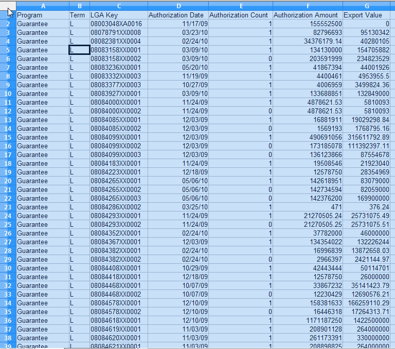
For this little exercise, we downloaded the file Export-Import Bank Authorizations for FY 2010

1. You open up a delimited or spreadhseet file of some sort either in Excel or OpenOffice Calc.
2. You click on the top left corner (or select the cells you want to copy). and use Ctrl+c or Edit->copy from menu.
   
3. Then you paste it into your Open Base window (preferably in Table section) that is connected to your PostgreSQL database.
   
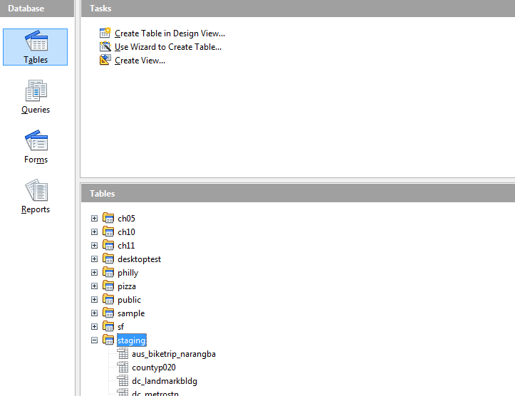
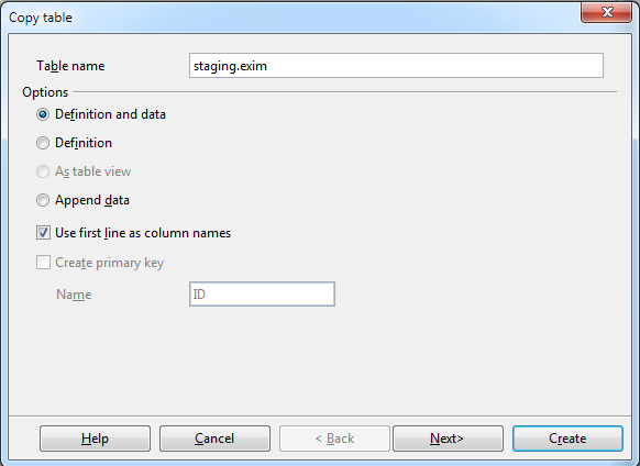
4. A wizard comes up asking you if you want to create a new table or append to an existing table. If you want to create a new table, give the table a name, preferably include the schema in the name. If you would have liked to append to a table, make sure you have the table selected before you start this whole copy paste routine.
   
   
5. Then the wizard guides you thru selecting the columns.
   
   
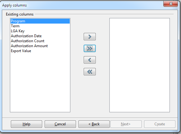
6. To which you have the option of selecting all with the >> or just some by holding the control key down, selecting the columns and then click >
   
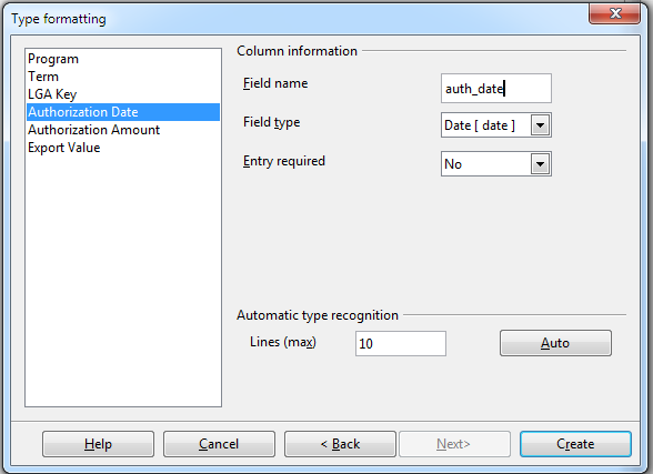
7. If you want to append to an existing table you get to map the fields. If a new you get to change the data types and names of the fields. Make sure to make them all lower case and no spaces to save yourself future grief.
   

Caveats

The SDBC driver is much more annoying than the JDBC driver for these exercises and we'll explain why. So short answer, you are probably better off using the latest PostgreSQL JDBC 4 driver.

• Open Office Base maintains the casing of the headers, so you will want to rename these to lower case either before import or during import. If you use the SDBC driver, it won't let you rename to lower case (it gives duplicate name error) if you simply try to lower case the column names, but JDBC works fine.
• By default for the JDBC driver, the data type of all the fields is set to TEXT, unless you change them which is okay for the most part, but for the SDBC driver it sets it to TEXT (char) which magically gets mapped to some non-existent data type that when it goes to create the table, fails horribly. To get around this annoyance, you have to change the data type of every single column to Text(Text) or some or TEXT (varchar) with the wizard before you import.
• Make sure to prefix new tables with the schema. we tried pasting using an account that had limited rights and it tried to create a table under a schema that didn't exist (presumably the users). which resulted in a create not allowed error.

In addition to all the new features in OpenOffice, we have a nice new shiny logo on the flash screen to remind us of who is boss. All hail to our new warlord and may the Oracle treat us well.

Other things you can do with Copy and Paste

• Copy a table and create a new table from it simply by pasting.
• Copy a table and append the contents to an existing table. In order to do this, first copy the table, then select the table you want to paste into, and then do a Ctrl-V to paste (or choose Edit->Paste from file menu)
• Copy a table and make it a view. Not quite sure why this is that useful since you can't edit the definition of the view in OO.